
LumoLabs website
We changed the layout of our site too.
LumoLabs is now at www.falklumo.com/lumolabs and hosts a repository of articles.
Therefore, we will use the blog to announce new articles or important updates to followers and interested parties. And to enable their discussion.
The actual articles are not posted as a blog article as its format was deemed unsuitable. But you'll find links to both the online article and a printable PDF version. If possible, we always recommend to download and read the PDF version. The PDF version does update more frequently too ;)
Understanding Image Sharpness
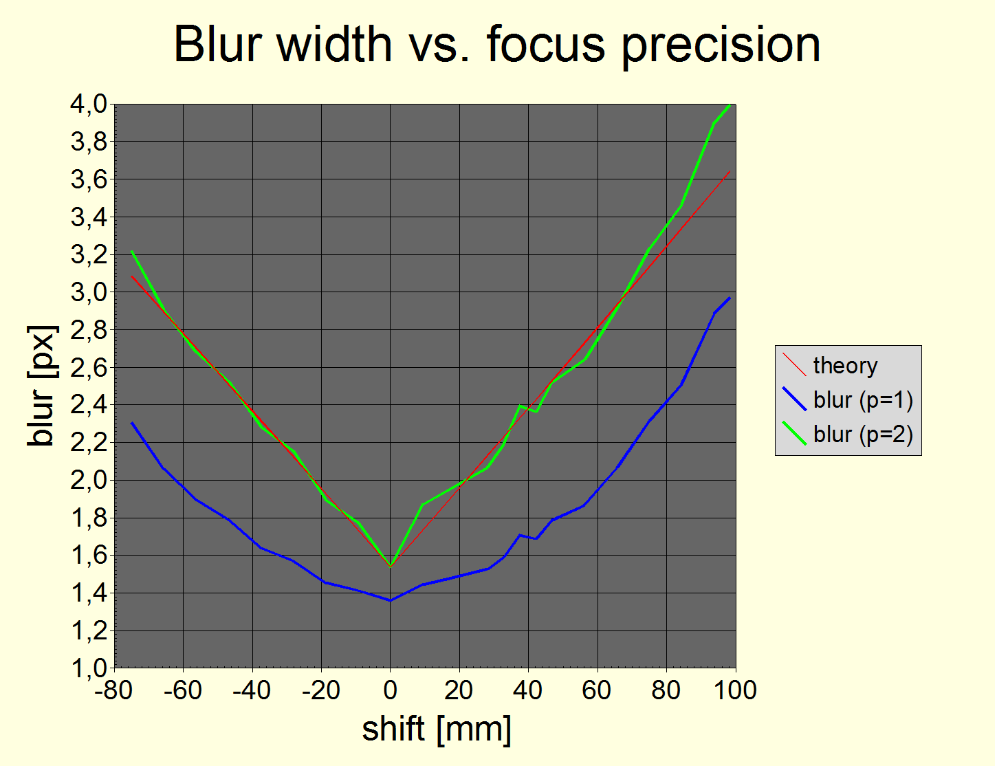
(Sample chart form the article)
Hint: The article image URLs actually open as larger images as they appear embedded in the article.
This article is a recommended read for anybody loving to dig into technology and who isn't afraid of a bit of math.
It's abstract and table of contents is:
Abstract
This White Paper is one in a series of articles discussing various aspects in obtaining sharp photographs such as obtaining sharp focus, avoiding shake and motion blur, possible lens resolution etc. This paper tries to provide a common basis for a quantitative discussion of these aspects.
Table of Content
1. Measures
1.1. Modular Transfer Function
1.2. Blur
1.2.1. The hard pixel
1.2.2. The perfect pixel
1.2.3. The real pixel, sharp and soft
1.3. More realistic resolution measures
1.4. Combining blur
2. Sources of blur
2.1. Defocus
2.1.1. Ability of deconvolution operators to reduce defocus blur
2.2. Bayer matrix and anti aliasing
2.3. Diffraction
2.4. Lens aberrations
2.4.1. Defocus, Spherical aberration, Coma, Astigmatism
2.5. Shake
2.5.1. Measuring shake
2.5.2. Expected shake
2.5.3. Empirical results
2.5.4. Tripod classification
2.6. Motion blur
2.7. Noise
2.8. Atmospheric perturbations
2.9. Precision and calibration
3. Practical considerations and examples
Please, proceed here:
- Online article (same as click onto blog title)
- PDF print version
Cooler Artikel - hab leider nur die Hälfte beim durchlesen verstandne... :-O
ReplyDeleteDie große Frage ist doch aber: Wie kann ich mit Haumittlen festellten, wie "scharf" mein Objektiv ist (bzw. beim Kauf beim freunldichen Händler da eben "schnell" testen)
lg, oli
oliver asks how to quick-test a lens.
ReplyDeleteWell, this article is meant to provide a common ground for forthcoming articles. An article about lens tests, both quick and more seriously, is in its planning stage.
Basically, if you photograph a dark gray surface's sharp border at a 5° angle (on a wall) with flash and use contrast-AF to focus (don't move ...), you're all set. Bring a piece of paper with a black square printed if your dealer doesn't happen to have it hanging on the wall...
And shoot RAW. Most importantly, always stick to constant development parameters. I heard that equal LR2 and LR3 sharpening parameters lead to different sharpenings, LR3 sharpening more.
Of course, you have to do this a couple of time sto develop some feeling to interpret results. And you need a tool like QuickMTF to actually measure something :)
This comment has been removed by the author.
ReplyDeleteManny, you can find my email address following to my web site (Falk Lumo's homepage). That may be a better way to ask for personal advice.
ReplyDeleteIn the particular case, it really depends what you are going to shoot. You don't actually need a system camera for baby and landscape. So, you really should test-drive all three and try to fall in love with one ;)
You may guess my love but not everybody loves the same way, fortunately :)
Hi Falk!
ReplyDeleteAre these 4 really the only comments so far? Strange! So here is the Matthias from NF-F, who just commented on one of your posts there.
I understand that the blur widths b in your model are not immediately comparable to the CoC of the classical DoF model. But if you were to combine various blur contributions into that DoF model, how would you combine them? I used an "RMS approach", but that was without having too much of a reason for it, or nothing more than the idea of adding up errors in statistics. Now that I see you do it similarly, but with much more of a reason, I feel a bit more secure with it. Is there any good reason NOT to do so?
So far I have diffraction blur and resolution ("pixel") blur combined into my DoF chart, but the relative scaling of those I could only guess. I am currently using the classical defocus CoC, 1/2 of the airy disc diameter and pixel pitch and simply sum up their squares. Would you have better ideas for their relative scalings?
2 days ago I started a discussion in another forum on how shake blur would be included in this model. So your appearance in the NF-F together with the link came perfectly in time. Different from defocus, diffraction and "pixel" blur, the one from shake is not circular. Of course even an uni-directional shake spoils your MTF, but is it also perceived like that by the human eye? After all, to produce a blur equivalent to e.g. diffraction would require the same shake in perpendicular directions at the same time. But during reasonably short exposure times you will probably get only a shake along one line. Is that perceived "as bad" as a circular CoC with the same diameter? Or is its effective "perceived diameter" smaller?
Gruß, Matthias
Hi Matthias,
ReplyDeletethis article appeared as a background article for another study and much of the discussion was over there, or at pentaxforums.com. But I agree, the article has enough potential for discussion, agreement and disagreement :)
Among other stuff, what I try to understand in my paper is how blur from different sources actually combines. I make no hard assumption here but come to the conclusion that it suffices to distinguish two types of blur: one with an S-shaped MTF curve and one with a more linear MTF-curve. And only the former type would combine using an "RMS approach" which I call the Kodak formula with p=2.
Interestingly, defocus blur (with a disc-shaped point spread function) seems to combine well with p=2, i.e., it's MTF should be S-shaped. I really have to do the math some day ;) OTOH, diffraction (with an Airy-disk shaped point spread function) is rather linear. However, my guess still is to use p=2 if there are S-shaped MTF curves involved, i.e., if the resulting MTF curve would be S-shaped.
About scaling ... you actually can't. You first would have to know the MTF of the Bayer demosaicing algorithm (which can only be simulated) and combine with analytical treatments of the pixel (in my paper), of the Bayer-AA filter (PSF is two/four Dirac peaks), of the defocus-MTF and of the diffraction-MTF (in my paper). Then, you can look up all MTF50 values and combine using an RMS approach (Kodak p=2 formula).
So, what I did in my paper is a measurement of MTF50 as a function of defocus with sharpening allowed to compsensate for Bayer-AA filtering. And use this as a base to discuss other sources of blur.
Falk,
ReplyDeletethanks for the immediate reply! Actually I am quite happy with my "RMS approach" now that I see that you come to a similar conclusion on a completely different path (at least for most blur contributors). But the big difference between your model and the classical DoF seems to be, that you are working with edge spread functions (do I remember correctly?), while DoF is all about point spread functions. Do they combine in a similar manner?
Obviously we can't know the blur from a particular sensor, AA-filter and demosaicing. But is that really necessary? Or can one guess it purely from the sensel pitch, perhaps with a +/- 20% error?
When you say you can't scale the contributions, why is that? I agree that the relative weightings might differ when looking at PSF rather than ESF. But I still stick to the idea to find an effectice diameter (or b in your case) by applying something like an RMS approach again and then summing up those effective areas (or use Kodak P=2).
I tried to do the maths for the MTF of a classical CoC, but got stuck somewhere. Google helped and I found it elsewhere. But where was that again???
Gruß, Matthias
@Matthias, it now becomes rather technical, so if you like, drop me an email (address found on homepage impressum).
DeleteWrt CoC MTF, there is a good source here:
http://www.scribd.com/doc/24288865/MTF-%E2%80%A2-Generally-Measure-MTF-Both-Horizontal-and-Vertical-I
showing a number of MTFs, incl. diffraction (same as in my paper) and defocus (with diffraction included). As you can see, defocus MTF becomes S-shaped for larger values of defocus but remains line-shaped for small defocus.
PSF vs. ESF vs. MTF ... It doesn't matter, because either function can be converted into any of the other two. E.g., PSF ist the derivative of ESF. Defining relative weightings is easy, just take the MTF50 values (the Kodak formula with p=2 allows to sum up the square of their inverse values). Computing MTF and the frequency of MTF=0.5 is the hard part, esp. for MTFs with no exact treatment like sharpened Bayer-sensor MTFs. In this case, I use values derived from measurements.
Erratum. LSF is the derivative of ESF, PSF is the two-dimensional variant of LSF.
Delete